Day 2 · About 6 hours, in three sessions
Prices over time
Download a share’s daily prices since 2016 and chart them, measure its returns day by day and year by year, and adjust raw prices for a split and a dividend.
Today’s goal
By the end of today you will have three programs. The first downloads a share’s daily prices, saves them, and draws this chart of its close:
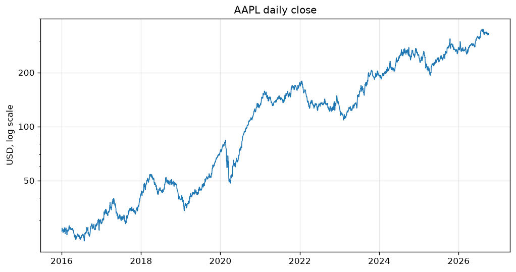
The second measures the share’s returns: its best and worst days, its growth a year, and each year’s return. The third finds a split in raw prices, adjusts for it, and counts a dividend in.
Why it matters on a desk
Every number a desk reports starts from a history of prices: how a strategy would have done, how risky a portfolio is, how a fund compares with the market. If the history is wrong, every number after it is wrong. A split read as a crash, or a dividend left out, changes the answer.
Returns are how a desk compares anything with anything: a share with the market, this year with last, a strategy with doing nothing. Today you work them out from the prices yourself, and learn to trust the prices first.
Review
A few questions from earlier days. Answer each before you start.
A share’s bid is 50.00 and its ask is 50.04. You buy 100 shares at once and sell them straight back. How much do you lose?
Show the answer
A: 4.00 dollars You pay the ask and get the bid back, so you lose the spread, 0.04, on each of the 100 shares: 100 × 0.04 = 4.00 dollars.
Which file lets anyone install exactly the same versions of your project’s packages?
Show the answer
C: uv.lock uv.lock records the exact version of every package. pyproject.toml lists the packages with the lowest versions that will do, and .venv is the installed copy that uv rebuilds from the lock file.
You changed a file and haven’t committed yet. Which command shows what you changed?
Show the answer
B: git diff git diff shows every line changed since the last commit. git log lists commits, and git revert undoes one.
Session 1 Daily prices since 2016, and a chart
The idea
Step 1 One day’s prices
Shares on the main US exchanges trade from 9:30 in the morning to 4:00 in the afternoon, New York time, on every weekday that isn’t a market holiday. A trading day’s prices are summed up in a bar of five numbers:
| Field | What it means | 6 Oct 2026, in the sample |
|---|---|---|
| open | The price the day opened at, at 9:30 | 327.10 |
| high | The highest price anyone paid that day | 331.05 |
| low | The lowest price anyone paid that day | 326.92 |
| close | The price the day closed at, at 16:00 | 330.27 |
| volume | How many shares changed hands | 41,250,310 |
Shares also trade before 9:30 and after 16:00, in smaller amounts, called pre-market and after-hours trading. The day’s volume counts those trades too, while its open, high, low and close are the main session’s.
Most analysis is built on the close: a day’s return, a year’s growth and the value of a portfolio are all worked out from closes.
Alpaca’s free plan has a daily bar for each symbol on every trading day since the start of 2016. Weekends and market holidays, such as Christmas Day, have none. The sample has 2,705 bars from 4 Jan 2016 to 6 Oct 2026.
Practice
Problem 1
2 pointsOne day’s bar has a high of 52.80 and a low of 51.10. What was the day’s range, the gap between its highest and lowest prices, in dollars?
Hint 1
The range is the gap between the two prices.
Hint 2
Take the low away from the high.
Solution
range = high − low
= 52.80 − 51.10
= 1.70 dollars
Problem 2
2 pointsOn a chart with a log scale, the step from 10 to 20 dollars is 3 cm tall. How tall, in cm, is the step from 100 to 400 dollars?
Hint 1
On a log scale, equal steps are equal percent moves. 10 to 20 is a doubling.
Hint 2
How many doublings take 100 to 400?
Solution
10 to 20 is one doubling, 3 cm
100 to 400 is 100 to 200, then 200 to 400: 2 doublings
2 × 3 cm = 6 cm
Which of a day’s prices is the one most analysis is built on?
Show the answer
B: The close The close is the day’s last price. Returns, growth and a portfolio’s value are all worked out from closes.
The project, step by step
Build it yourself from this brief, then check it against the steps.
- Add pandas and matplotlib to the market-data project, and add
data/andcharts/to.gitignore. - Make alpaca.py, a module for Alpaca’s market data API: its base address,
https://data.alpaca.markets, written once; one httpx2 client for every request, made the first time it is needed, that sends your keys;snapshots(symbols);bars(symbol, query), which asks/v2/stocks/barspage by page until there is nonext_page_token;day_of(timestamp), the New York date of one of Alpaca’s UTC times; anddaily_bars(symbol), every day since 2016, adjusted for splits. Make quote.py and watchlist.py use it. - Write history.py. It takes a ticker from the command line, AAPL if there is none, and turns
alpaca.daily_barsinto a DataFrame of open, high, low, close and volume with the dates as its index, oldest first. - It prints the last five days, how many days there are with the first and last date, and the highest close with its date.
- It saves the table to
data/AAPL.csvand a chart of the close, on a log scale, tocharts/AAPL.png(with the ticker in place of AAPL). - Run it for AAPL and for SPY, then commit.
Step 1 Add pandas and matplotlib
pandas works with tables of data, and matplotlib draws charts. In the market-data folder, add both:
uv add pandas matplotlibResolved 22 packages in 333msDownloading numpy (15.9MiB)Downloading pillow (6.6MiB)Downloading kiwisolver (1.4MiB)Downloading pandas (10.3MiB)Downloading fonttools (5.1MiB)Downloading matplotlib (10.4MiB) Downloaded kiwisolver Downloaded fonttools Downloaded pillow Downloaded pandas Downloaded matplotlib Downloaded numpyPrepared 12 packages in 2.18sInstalled 12 packages in 197ms + contourpy==1.4.0 + cycler==0.12.1 + fonttools==4.66.1 + kiwisolver==1.5.1 + matplotlib==3.11.2 + numpy==2.5.3 + packaging==26.3 + pandas==3.0.6 + pillow==12.3.0 + pyparsing==3.3.3 + python-dateutil==2.9.0.post0 + six==1.17.0cat pyproject.toml[project]name = "market-data"version = "0.1.0"description = "US equity market data in Python"readme = "README.md"requires-python = ">=3.14"dependencies = [ "httpx2>=2.13.1", "matplotlib>=3.11.2", "pandas>=3.0.6",]
uv also installed the packages they need, such as numpy, which does arithmetic on a whole column at once. Both are now listed in
pyproject.tomlunder dependencies.Step 2 Download the history
Make a new file, history.py, and type this in:
history.pyimport os import httpx2import pandas as pd url = "https://data.alpaca.markets/v2/stocks/bars"keys = { "APCA-API-KEY-ID": os.environ["APCA_API_KEY_ID"], "APCA-API-SECRET-KEY": os.environ["APCA_API_SECRET_KEY"],}query = { "symbols": "AAPL", "timeframe": "1Day", "start": "2016-01-01", "adjustment": "split", "feed": "sip", "limit": 10000,}response = httpx2.get(url, params=query, headers=keys, timeout=30)bars = response.json()["bars"]["AAPL"]prices = pd.DataFrame(bars)print(prices.head())print(len(prices), "rows")- Line 4
- Load pandas under the short name everyone uses,
pd. - Line 6
- The address of Alpaca’s bars.
- Lines 7 to 10
- Your keys, as on Day 1.
- Lines 11 to 18
- Apple’s bars, one a day (
1Day), from the start of 2016, adjusted for splits (Session 3 explains it), from every US exchange (sip), up to 10,000 in one answer, the most Alpaca sends. - Line 19
- Ask for them.
timeout=30waits up to 30 seconds, since a history is much longer than a quote. - Line 20
- The answer holds the bars by symbol, so
["bars"]["AAPL"]is Apple’s list, a dictionary for each day. - Line 21
pd.DataFrameturns the list into a table: a row for each dictionary, and a column for each name in them.- Line 22
head()is the table’s first five rows.- Line 23
lencounts the rows: one for each trading day.
uv run --env-file .env history.py c h l ... t v vw0 26.11 26.25 26.02 ... 2016-01-04T05:00:00Z 134757189 26.14331 26.41 26.45 26.01 ... 2016-01-05T05:00:00Z 267481579 26.27862 27.17 27.36 26.33 ... 2016-01-06T05:00:00Z 179862001 26.88533 26.57 27.54 26.52 ... 2016-01-07T05:00:00Z 231609206 26.88934 26.74 26.86 26.45 ... 2016-01-08T05:00:00Z 189244654 26.6676 [5 rows x 8 columns]2705 rows
Shown for the course’s sample data. Yours shows the latest.
Column What it is o, h, l, c The day’s open, high, low and close v The volume: how many shares traded n How many trades there were vw The volume-weighted average price, which Day 3 explains t The time the bar starts, in UTC pandas leaves out columns from the middle, marked
..., when a table is wider than the terminal. The numbers down the left, 0 to 4, are the index pandas gave the rows: their positions. Each day’s bar starts at midnight in New York, which Alpaca writes in UTC: 05:00 in winter, when New York is 5 hours behind. The next step makes the New York dates the index.Look at the volume in 2016: 134,757,189 shares on the first day. Session 3 explains why it is so large.
Step 3 A client module for Alpaca
quote.py and history.py both ask Alpaca, at addresses that start the same way, with the same keys. Rather than repeat that, and the code that asks, in every file that needs it, give Alpaca a module of its own, and import from it everywhere else. A change to how you reach Alpaca is then made in one place.
Make alpaca.py:
alpaca.py"""Alpaca's market data: snapshots and daily bars. Snapshots are 15 minutes behind the market and cover every US exchange. The freeplan has bars since 2016, up to 15 minutes ago. The data is for personal use.""" import osfrom datetime import datetimefrom functools import lru_cachefrom zoneinfo import ZoneInfo import httpx2 BASE_URL = "https://data.alpaca.markets"# The market's time zone. Alpaca gives every time in UTC.NEW_YORK = ZoneInfo("America/New_York") @lru_cachedef client(): """One client for every request to Alpaca, made the first time it is needed: it keeps its connection open between requests and sends your keys with each.""" keys = { "APCA-API-KEY-ID": os.environ["APCA_API_KEY_ID"], "APCA-API-SECRET-KEY": os.environ["APCA_API_SECRET_KEY"], } return httpx2.Client(base_url=BASE_URL, headers=keys, timeout=10) def get(path, params): """GET a path with its query and return the JSON.""" response = client().get(path, params=params) response.raise_for_status() return response.json() def snapshots(symbols): """Each symbol's latest trade, quote and daily bars, 15 minutes behind.""" query = {"symbols": ",".join(symbols), "feed": "delayed_sip"} return get("/v2/stocks/snapshots", query) def bars(symbol, query): """A symbol's bars, oldest first, following Alpaca's pages to the last.""" query = {"symbols": symbol, "feed": "sip", "limit": 10000, **query} found = [] while True: page = get("/v2/stocks/bars", query) found += page["bars"].get(symbol, []) if not page["next_page_token"]: return found query["page_token"] = page["next_page_token"] def day_of(timestamp): """The New York date of one of Alpaca's UTC times.""" return datetime.fromisoformat(timestamp).astimezone(NEW_YORK).date() def daily_bars(symbol): """Every trading day's bar since 2016, adjusted for splits.""" query = {"timeframe": "1Day", "start": "2016-01-01", "adjustment": "split"} return bars(symbol, query)- Line 14
- The start every Alpaca address shares, written once.
- Line 16
- The market’s time zone, by its name in the world’s time-zone database, which knows when each zone changes its clocks.
zoneinfocomes with Python. - Lines 19 to 27
@lru_cacheis a decorator: it wraps the function below it so that the first call runs it and keeps the answer, and every call after returns that same answer. Soclient()makes one client, the first time a request needs it, and reads your keys then, not when the file is imported. A client sends every request with the same settings, the base address, your keys and a 10-second timeout, and keeps its connection to Alpaca open between requests, which is faster than connecting each time.- Lines 30 to 34
- Ask for a path under the base address with a query, stop with an error if the server answered with a problem, and return the JSON.
- Lines 37 to 40
- Snapshots for a list of symbols: Day 1’s request, now in one place.
- Lines 43 to 52
- Alpaca sends at most
limitbars in one answer, called a page. When there are more, the answer’snext_page_tokenis set, and sending it back aspage_tokengets the next page. Thewhile Trueloop asks, adds the page’s bars tofound, and stops when there is no token.**querycopies the caller’s query into the new dictionary after the three settings every request shares. - Lines 55 to 57
datetime.fromisoformatreads a time such as 2016-01-04T05:00:00Z,astimezone(NEW_YORK)gives the same moment in New York’s time, and.date()keeps its date.- Lines 60 to 63
- Every day since the start of 2016, adjusted for splits: history-1.py’s request, now in one place.
Make quote.py use it. The download code moves out, and
alpaca.snapshotstakes its place:quote.py"""Print a stock's latest quote from Alpaca, 15 minutes behind the market. Run it with a ticker, such as: uv run --env-file .env quote.py AAPL""" import sys import alpaca def describe(symbol, snapshot): """One line about a symbol: its last price, bid, ask and spread.""" last = snapshot["latestTrade"]["p"] bid = snapshot["latestQuote"]["bp"] ask = snapshot["latestQuote"]["ap"] return ( f"{symbol} last {last:.2f} bid {bid:.2f} ask {ask:.2f} " f"spread {ask - bid:.2f}" ) if __name__ == "__main__": symbol = sys.argv[1] if len(sys.argv) > 1 else "AAPL" snapshots = alpaca.snapshots([symbol]) if symbol not in snapshots: sys.exit(f"No quote for {symbol}: check the ticker.") print(describe(symbol, snapshots[symbol]))- Line 10
- Import the module, and call its functions by its name, as
alpaca.snapshots. Each call then says where its data comes from.
And watchlist.py:
watchlist.py"""A watchlist: the latest quotes for a few symbols, refreshed every minute. Run it, and press Ctrl+C to stop: uv run --env-file .env watchlist.py""" import timefrom datetime import datetime import alpaca SYMBOLS = ["AAPL", "MSFT", "NVDA", "SPY", "QQQ"]REFRESH_SECONDS = 60 def row(symbol, snapshot): """One table row: symbol, last price, and change since the previous close.""" last = snapshot["latestTrade"]["p"] previous = snapshot["prevDailyBar"]["c"] change = last - previous return f"{symbol:<6} {last:>10.2f} {change:>+8.2f} {change / previous:>+8.2%}" def show(symbols): """Print the time, a header, then one row per symbol, from one request.""" snapshots = alpaca.snapshots(symbols) print(f"\nQuotes at {datetime.now():%H:%M:%S}") print(f"{'symbol':<6} {'last':>10} {'change':>8} {'%':>8}") for symbol in symbols: print(row(symbol, snapshots[symbol])) if __name__ == "__main__": try: while True: show(SYMBOLS) time.sleep(REFRESH_SECONDS) except KeyboardInterrupt: print("\nStopped.")quote.py prints what it printed before:
uv run --env-file .env quote.pyAAPL last 330.27 bid 330.25 ask 330.30 spread 0.05
Shown for the course’s sample data. Yours shows the latest.
Step 4 Make the dates the index
Replace history.py with this. The new and changed lines are marked:
history.pyimport pandas as pd import alpaca # Alpaca's short names for a bar's fields, and the names this project uses.COLUMNS = {"o": "open", "h": "high", "l": "low", "c": "close", "v": "volume"} def get_history(symbol): """Every trading day's open, high, low, close and volume since 2016, adjusted for splits, oldest first, dated.""" bars = alpaca.daily_bars(symbol) prices = pd.DataFrame(bars, columns=list(COLUMNS)).rename(columns=COLUMNS) prices.index = pd.DatetimeIndex( [alpaca.day_of(bar["t"]) for bar in bars], name="date" ) return prices prices = get_history("AAPL")print(prices.tail())first, last = prices.index[0], prices.index[-1]print(f"\n{len(prices):,} days, from {first:%d %b %Y} to {last:%d %b %Y}")high = prices["close"].idxmax()print(f"highest close: {prices['close'].max():.2f} on {high:%d %b %Y}")- Line 3
- alpaca.py, beside history.py, is imported like any package.
- Line 6
- A dictionary from Alpaca’s short names to the names this project uses, for the five columns today’s code needs.
- Lines 9 to 12
- A function that turns a symbol’s daily bars into a table. Its docstring, the lines in triple quotes under
def, says what it returns. - Line 13
columns=list(COLUMNS)keeps only the five fields COLUMNS names, in its order, andrenameswaps each short name for its long one. With no bars, as for a ticker Alpaca doesn’t know, it makes an empty table with those columns.- Lines 14 to 15
alpaca.day_ofturns each bar’s time into its New York date, andpd.DatetimeIndexmakes the dates the index, nameddate. Alpaca sends bars oldest first, so they are in order already.- Lines 20 to 21
- Fetch Apple’s history and print its last five rows:
tail()is the end of the table, ashead()is its start. - Lines 22 to 23
prices.index[0]is the first date andprices.index[-1]the last: a minus counts from the end.\nstarts with an empty line,:,writes the count with commas, and:%d %b %Ywrites a date as its day, month and year, such as 06 Oct 2026.- Lines 24 to 25
idxmax()gives the index of the largest value: the date of the highest close.max()gives the value. Inside the f-string the column’s name is in single quotes,prices['close'], because the f-string itself is in double quotes.
uv run --env-file .env history.py open high low close volumedate 2026-09-30 329.56 329.67 322.46 324.62 402199282026-10-01 325.15 333.11 324.50 330.70 313314322026-10-02 331.85 333.52 329.35 330.32 292848752026-10-05 329.73 330.36 325.61 326.80 547217272026-10-06 327.10 331.05 326.92 330.27 41250310 2,705 days, from 04 Jan 2016 to 06 Oct 2026highest close: 349.26 on 17 Aug 2026
Shown for the course’s sample data. Yours shows the latest.
The dates now run down the left as the index.
datesits on a line of its own above them because it names the index, not a column.Yours will show real prices. Run during a trading day, the last row is the day so far, 15 minutes behind, and it changes until the day closes. And a real price can have up to four decimal places: some trades are matched at fractions of a cent, such as halfway between the bid and the ask.
Step 5 Keep the data out of Git
The next step saves Alpaca’s prices in a folder called data, and charts of them in a folder called charts. Alpaca’s data is for your own use, and on Day 4 your repository goes on GitHub for anyone to see, so keep both folders out of Git.
Open
.gitignorein VS Code and add three lines at its end: a comment, thendata/andcharts/. A line starting with # is a comment, a note for people that Git skips. Then print the file to check it:cat .gitignore# Python-generated files__pycache__/*.py[oc]build/dist/wheels/*.egg-info # Virtual environments.venv # Downloaded prices, and the charts made from themdata/charts/ # Your API keys and other settings for this computer only.env
Step 6 Save the prices, and chart them
Replace history.py with this:
history.py"""Download a share's daily prices since 2016, save them, and chart the close. Run it with a ticker, such as: uv run --env-file .env history.py AAPL""" import sysfrom pathlib import Path import matplotlib.pyplot as pltimport pandas as pdfrom matplotlib import ticker import alpaca # Alpaca's short names for a bar's fields, and the names this project uses.COLUMNS = {"o": "open", "h": "high", "l": "low", "c": "close", "v": "volume"} def get_history(symbol): """Every trading day's open, high, low, close and volume since 2016, adjusted for splits, oldest first, dated.""" bars = alpaca.daily_bars(symbol) prices = pd.DataFrame(bars, columns=list(COLUMNS)).rename(columns=COLUMNS) prices.index = pd.DatetimeIndex( [alpaca.day_of(bar["t"]) for bar in bars], name="date" ) return prices def chart(prices, symbol, path): """The close on every day, on a log scale, saved as a picture.""" fig, ax = plt.subplots(figsize=(10, 5)) ax.plot(prices.index, prices["close"], linewidth=1) ax.set_yscale("log") ax.yaxis.set_major_locator(ticker.LogLocator(subs=[1, 2, 5])) ax.yaxis.set_major_formatter(ticker.StrMethodFormatter("{x:,g}")) ax.yaxis.set_minor_formatter(ticker.NullFormatter()) ax.grid(alpha=0.3) ax.set_title(f"{symbol} daily close") ax.set_ylabel("USD, log scale") fig.savefig(path, dpi=120, bbox_inches="tight") if __name__ == "__main__": symbol = sys.argv[1] if len(sys.argv) > 1 else "AAPL" prices = get_history(symbol) if prices.empty: sys.exit(f"No prices for {symbol}: check the ticker.") print(prices.tail()) first, last = prices.index[0], prices.index[-1] print(f"\n{len(prices):,} days, from {first:%d %b %Y} to {last:%d %b %Y}") high = prices["close"].idxmax() print(f"highest close: {prices['close'].max():.2f} on {high:%d %b %Y}") Path("data").mkdir(exist_ok=True) Path("charts").mkdir(exist_ok=True) prices.to_csv(f"data/{symbol}.csv") chart(prices, symbol, f"charts/{symbol}.png") print(f"saved data/{symbol}.csv and charts/{symbol}.png")- Lines 1 to 6
- A docstring for the whole file: what it does and how to run it.
- Lines 8 to 13
- New imports:
sysfor the command line,Pathfor making folders, matplotlib’spyplot(asplt, its usual short name) for drawing, andtickerfor the numbers on the price scale. - Lines 32 to 35
plt.subplotsmakes a figure, the whole picture, 10 by 5 inches, and the axes inside it, which is the chart itself.ax.plotdraws the close against the dates, as a line 1 point wide.- Line 36
- Put the price scale on a log scale.
- Lines 37 to 39
- Mark the scale at 1, 2 and 5 times each power of 10 (2, 5, 10, 20, 50, 100 and so on), write those marks as plain numbers, and leave the small marks between them unlabelled. Without these lines, matplotlib labels a log scale in powers of 10, such as 10², which is hard to read.
- Line 40
- Faint lines across the chart at each labelled price, to read it by.
alpha=0.3makes them 30% opaque. - Lines 41 to 42
- The chart’s title, and the label of its price scale.
- Line 43
- Save the picture at 120 dots for each inch, so 1,200 by 600 pixels, trimmed to the chart by
bbox_inches="tight". - Lines 46 to 48
- Only when the file is run: take the ticker from the command line, AAPL if there is none, and fetch its history.
- Lines 49 to 50
- An empty table means Alpaca has no prices for that ticker, so say so and stop, as quote.py does. The printing that follows is as before, one level in.
- Lines 56 to 57
- Make the data and charts folders.
exist_ok=Truemeans it is fine if they are already there. - Line 58
- Save the table as CSV, comma-separated values: plain text with a line for each day, which pandas, Excel and nearly every other tool can read.
- Lines 59 to 60
- Draw the chart into the charts folder, and say where both files went.
uv run --env-file .env history.py AAPL open high low close volumedate 2026-09-30 329.56 329.67 322.46 324.62 402199282026-10-01 325.15 333.11 324.50 330.70 313314322026-10-02 331.85 333.52 329.35 330.32 292848752026-10-05 329.73 330.36 325.61 326.80 547217272026-10-06 327.10 331.05 326.92 330.27 41250310 2,705 days, from 04 Jan 2016 to 06 Oct 2026highest close: 349.26 on 17 Aug 2026saved data/AAPL.csv and charts/AAPL.png
Shown for the course’s sample data. Yours shows the latest.
Open
charts/AAPL.pngin VS Code:Shown for the course’s sample data. Yours shows the latest. Each labelled step up the scale is a doubling: 50 to 100 is as tall as 100 to 200. Now chart SPY, the fund that follows the S&P 500 from Day 1:
uv run --env-file .env history.py SPY open high low close volumedate 2026-09-30 762.17 764.63 761.44 762.10 398148862026-10-01 761.29 769.92 756.97 769.24 369522762026-10-02 769.44 775.45 768.88 772.77 384907602026-10-05 771.52 773.91 766.81 767.20 442552822026-10-06 768.05 772.10 767.80 771.53 52310998 2,705 days, from 04 Jan 2016 to 06 Oct 2026highest close: 773.49 on 06 Aug 2026saved data/SPY.csv and charts/SPY.png
Shown for the course’s sample data. Yours shows the latest.
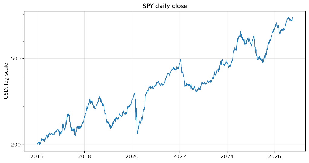
Shown for the course’s sample data. Yours shows the latest. The sample follows the market’s real path. SPY fell by about a third in a month in early 2020, when Covid-19 shut much of the world, and by about a quarter through most of 2022, as interest rates rose.
Step 7 Commit your work
git statusOn branch mainChanges not staged for commit: (use "git add <file>..." to update what will be committed) (use "git restore <file>..." to discard changes in working directory) modified: .gitignore modified: pyproject.toml modified: quote.py modified: uv.lock modified: watchlist.py Untracked files: (use "git add <file>..." to include in what will be committed) alpaca.py history.py no changes added to commit (use "git add" and/or "git commit -a")git add .git commit -m "Add an Alpaca client, and save and chart daily prices"[main e4d46e6] Add an Alpaca client, and save and chart daily prices 7 files changed, 567 insertions(+), 20 deletions(-) create mode 100644 alpaca.py create mode 100644 history.py
git statuslists your two new files, alpaca.py and history.py, and the five that you anduv addchanged, but not the data or charts folders:.gitignorekeeps them out.
Session 2 Returns: daily, total and yearly
The idea
Step 1 A day’s return
A return measures a move as a share of where the price started. In words, a day’s return is its close divided by the day before’s close, minus 1. Times 100, it is a percent.
| Day | Close | Return = close ÷ day before’s close − 1 |
|---|---|---|
| 30 Sep 2026 | 324.62 | the first day shown |
| 1 Oct 2026 | 330.70 | 330.70 ÷ 324.62 − 1 = 0.018730, or +1.87% |
| 2 Oct 2026 | 330.32 | 330.32 ÷ 330.70 − 1 = -0.001149, or −0.11% |
| 5 Oct 2026 | 326.80 | 326.80 ÷ 330.32 − 1 = -0.010656, or −1.07% |
| 6 Oct 2026 | 330.27 | 330.27 ÷ 326.80 − 1 = 0.010618, or +1.06% |
Returns, not dollar changes, are what a desk compares. A move of 3 dollars is a large one for a 30-dollar share and a small one for a 3,000-dollar share.
pct_change() works out every day’s return at once. The first day has no day before it, so its return is missing: pandas marks it NaN, short for “not a number”, and dropna() drops it.
Practice
Problem 3
2 pointsA share closed at 40.00 yesterday and at 41.00 today. What was today’s return, in percent?
Hint 1
A return is today’s close ÷ yesterday’s close − 1.
Hint 2
Multiply by 100 to make it a percent.
Solution
return = 41.00 ÷ 40.00 − 1
= 1.025 − 1 = 0.025
= 2.5%
Problem 4
2 pointsA share rises 25% one day and falls 20% the next. What is its return over the two days, in percent?
Hint 1
Returns multiply. Each dollar becomes 1 + r dollars each day.
Hint 2
Multiply 1.25 by 0.80, then take away 1.
Solution
total = (1 + 0.25) × (1 − 0.20) − 1
= 1.25 × 0.80 − 1
= 1.00 − 1 = 0
So 0%: the share is back where it started.
Problem 5
2 pointsA fund grew from 100.00 to 200.00 in exactly 10 years. What was its growth a year, compounded, in percent?
Hint 1
Growth a year = (last ÷ first) to the power 1 ÷ years, minus 1.
Hint 2
(200.00 ÷ 100.00) is 2. Raise it to the power 1 ÷ 10, which is 0.1.
Solution
growth a year = (200.00 ÷ 100.00) to the power 1 ÷ 10, minus 1
= 2 to the power 0.1, minus 1
= 1.0718 − 1 = 0.0718
= 7.18% a year
returns.py divides the days between the first and last date by 365.25. Why 365.25?
Show the answer
C: It is the average number of days in a year, counting a leap day every fourth year The days counted are calendar days, weekends and holidays included, so dividing by the average length of a calendar year gives years. A year has about 252 trading days.
The project, step by step
Build it yourself from this brief, then check it against the steps.
- Write returns.py. It reads
data/AAPL.csv, which history.py saved, with the dates as the index (or another ticker’s file, given on the command line). - It prints the best and worst day’s return with their dates, the first and last close, the total return, and the growth a year, compounded.
- It ends with a table of each calendar year’s return, from one year’s last close to the next’s.
- Run it for AAPL and SPY, then commit.
Step 1 Each day’s return
Make returns.py beside history.py:
returns.pyimport pandas as pd prices = pd.read_csv("data/AAPL.csv", index_col="date", parse_dates=True)close = prices["close"]daily = close.pct_change().dropna()print(daily.tail())print(f"\nbest day: {daily.max():+.2%} on {daily.idxmax():%d %b %Y}")print(f"worst day: {daily.min():+.2%} on {daily.idxmin():%d %b %Y}")- Line 3
- Read the CSV that history.py saved.
index_col="date"makes the date column the index again, andparse_dates=Truereads its dates as dates, not text. - Line 4
- The close column, a Series: a value for each date.
- Line 5
pct_change()works out each day’s return. The first day has none, sodropna()drops it.- Line 6
- The last five days’ returns, as fractions.
- Lines 7 to 8
:+.2%writes a fraction as a percent, with its sign and two decimal places: 0.022529 becomes +2.25%.idxmin()gives the date of the smallest value, asidxmax()gives the largest’s. The two spaces after “best day:” line the numbers up.
uv run returns.pydate2026-09-30 -0.0141822026-10-01 0.0187302026-10-02 -0.0011492026-10-05 -0.0106562026-10-06 0.010618Name: close, dtype: float64 best day: +11.76% on 10 Mar 2020worst day: -11.15% on 18 Mar 2020
Shown for the course’s sample data. Yours shows the latest.
The returns print as fractions: -0.001149 is 0.11%.
Name: closesays which column the Series came from, anddtype: float64says its values are decimal numbers.Step 2 Total return, and growth a year
Replace returns.py with this:
returns.pyimport pandas as pd def load(symbol): """The prices history.py saved, dated.""" return pd.read_csv(f"data/{symbol}.csv", index_col="date", parse_dates=True) def daily_returns(close): """Each day's return: today's close over yesterday's, minus 1.""" return close.pct_change().dropna() def total_return(close): """The whole period's return: the last close over the first, minus 1.""" return close.iloc[-1] / close.iloc[0] - 1 def yearly_growth(close): """The growth each year that, compounded, gives the total return.""" years = (close.index[-1] - close.index[0]).days / 365.25 return (close.iloc[-1] / close.iloc[0]) ** (1 / years) - 1 close = load("AAPL")["close"]daily = daily_returns(close)print(f"best day: {daily.max():+.2%} on {daily.idxmax():%d %b %Y}")print(f"worst day: {daily.min():+.2%} on {daily.idxmin():%d %b %Y}")print(f"from {close.iloc[0]:.2f} to {close.iloc[-1]:.2f}")print(f"total return: {total_return(close):+,.1%}")print(f"growth a year, compounded: {yearly_growth(close):+.1%}")- Lines 4 to 6
- Read a symbol’s CSV, as before, now in a function.
- Lines 9 to 11
- Each day’s return, as before.
- Lines 14 to 16
ilocpicks a value by its position:iloc[0]is the first close andiloc[-1]the last. The total return is the last ÷ the first − 1.- Lines 19 to 22
- Taking the first date from the last gives the time between them, and
.dayscounts it in days. Dividing by 365.25 turns days into years, and** (1 / years)raises the ratio to the power 1 ÷ years. - Lines 25 to 26
- Load Apple’s prices, take the close, and work out its daily returns.
- Lines 29 to 31
- Print the first and last close, the total return and the growth a year.
:+,.1%is a percent with its sign, thousands separated by commas, and one decimal place.
uv run returns.pybest day: +11.76% on 10 Mar 2020worst day: -11.15% on 18 Mar 2020from 26.11 to 330.27total return: +1,164.9%growth a year, compounded: +26.6%
Shown for the course’s sample data. Yours shows the latest.
Step 3 Each calendar year
Replace returns.py with the finished file. It takes a ticker from the command line, and adds a year-by-year table:
returns.py"""Daily, total and yearly returns of a share, from the prices history.py saved. Run it with a ticker, such as: uv run returns.py AAPL""" import sys import pandas as pd def load(symbol): """The prices history.py saved, dated.""" return pd.read_csv(f"data/{symbol}.csv", index_col="date", parse_dates=True) def daily_returns(close): """Each day's return: today's close over yesterday's, minus 1.""" return close.pct_change().dropna() def total_return(close): """The whole period's return: the last close over the first, minus 1.""" return close.iloc[-1] / close.iloc[0] - 1 def yearly_growth(close): """The growth each year that, compounded, gives the total return.""" years = (close.index[-1] - close.index[0]).days / 365.25 return (close.iloc[-1] / close.iloc[0]) ** (1 / years) - 1 def calendar_years(close): """Each calendar year's return, from one year's last close to the next's.""" return close.resample("YE").last().pct_change().dropna() if __name__ == "__main__": symbol = sys.argv[1] if len(sys.argv) > 1 else "AAPL" close = load(symbol)["close"] daily = daily_returns(close) print(f"best day: {daily.max():+.2%} on {daily.idxmax():%d %b %Y}") print(f"worst day: {daily.min():+.2%} on {daily.idxmin():%d %b %Y}") print(f"from {close.iloc[0]:.2f} to {close.iloc[-1]:.2f}") print(f"total return: {total_return(close):+,.1%}") print(f"growth a year, compounded: {yearly_growth(close):+.1%}") print("\nyear return") for year, r in calendar_years(close).items(): print(f"{year:%Y} {r:+7.1%}")- Lines 1 to 6
- The file’s docstring.
- Lines 34 to 36
resample("YE")groups the days by calendar year, each group ending at the year’s end (YE)..last()keeps each year’s last close.pct_change()then gives each year’s return from the year before’s last close, anddropna()drops the first year, which has no year before it in the data.- Lines 39 to 41
- Take the ticker from the command line, AAPL if there is none.
- Lines 48 to 50
- A header, then a row for each year.
.items()gives each year’s date with its return.{year:%Y}writes the year alone, and{r:+7.1%}the return with its sign, in 7 characters, so the column lines up.
uv run returns.py AAPLbest day: +11.76% on 10 Mar 2020worst day: -11.15% on 18 Mar 2020from 26.11 to 330.27total return: +1,164.9%growth a year, compounded: +26.6% year return2017 +46.1%2018 -6.8%2019 +86.2%2020 +80.7%2021 +33.8%2022 -26.4%2023 +48.2%2024 +30.7%2025 +8.6%2026 +21.3%
Shown for the course’s sample data. Yours shows the latest.
uv run returns.py SPYbest day: +9.42% on 10 Mar 2020worst day: -10.40% on 18 Mar 2020from 201.15 to 771.53total return: +283.6%growth a year, compounded: +13.3% year return2017 +19.4%2018 -6.2%2019 +28.9%2020 +16.2%2021 +26.9%2022 -19.5%2023 +24.3%2024 +23.3%2025 +16.6%2026 +12.6%
Shown for the course’s sample data. Yours shows the latest.
The last row is the year so far: the sample ends on 6 Oct. In 2022, as interest rates rose, both fell: −26.4% and −19.5%. In other years a share can do far better or far worse than the market: in 2020 the sample’s AAPL returned +80.7% against SPY’s +16.2%.
Step 4 Commit your work
git add returns.pygit commit -m "Measure daily, total and yearly returns"[main 8ad5505] Measure daily, total and yearly returns 1 file changed, 50 insertions(+) create mode 100644 returns.py
Session 3 Splits and dividends: adjusted prices
The idea
Step 1 Stock splits
A stock split gives each owner more shares, each worth less, so that what they own is worth the same. In a 4-for-1 split each share becomes 4 shares, and the price is divided by 4.
Companies split when their share price has grown high, so that one share costs less to buy. Apple has split five times since it first sold shares in 1980, most recently 4 for 1 in August 2020.
A raw price history shows each day’s price as it was that day. On a split day it falls off a cliff. The sample company’s raw close went from 405.57 on 14 Jul to 101.61 on 15 Jul, a fall of 74.95% that cost no owner anything.
Practice
Problem 6
2 pointsA share at 300.00 splits 3 for 1. What is its price just after the split, if nothing else changes?
Hint 1
Each share becomes 3 shares, and what an owner holds is worth the same.
Hint 2
Divide the price by 3.
Solution
price after = price before ÷ ratio
= 300.00 ÷ 3
= 100.00
Problem 7
2 pointsBefore a 5-for-1 split you own 8 shares at 250.00. How many shares do you own after it?
Hint 1
Each of your shares becomes 5.
Hint 2
Multiply your 8 shares by 5.
Solution
shares after = shares before × ratio
= 8 × 5 = 40 shares
each worth 250.00 ÷ 5 = 50.00, so 40 × 50.00 = 2,000.00, as before
Problem 8
2 pointsA share closed at 50.00. The next day was its ex-dividend day, for a dividend of 0.50 a share, and it closed at 49.75. What was that day’s total return, in percent?
Hint 1
A day’s total return = (close + dividend) ÷ yesterday’s close − 1.
Hint 2
Add the 0.50 to 49.75 before you divide by 50.00.
Solution
total return = (49.75 + 0.50) ÷ 50.00 − 1
= 50.25 ÷ 50.00 − 1
= 1.005 − 1 = 0.005
= 0.5%
history.py asks Alpaca for adjustment=split. Its history is adjusted for which of these?
Show the answer
A: Splits, but not dividends Its prices before each split are divided by the split’s ratio, so a split never shows as a fall. Dividends are not in it, so its returns are price returns.
The project, step by step
Build it yourself from this brief, then check it against the steps.
- Download the raw sample,
https://sulba.dev/days/split-sample.csv, into your data folder. - Write adjust.py. It reads the sample with its dates as the index, finds each split from the close (a fall of more than half in a day) with its ratio, and adjusts every close, dividend and volume before it.
- It prints each split, the first and last adjusted close, the price return, and the total return with the dividend counted in.
- It also looks for splits in your
data/AAPL.csv. There should be none, because history.py asked for it adjusted.
Step 1 Download the raw sample
The raw sample is a month of a sample company’s prices, not adjusted: each day’s close, its volume, and the dividend paid on it, if any. Download it into your data folder:
Windows
curl.exe -o data/split-sample.csv https://sulba.dev/days/split-sample.csvmacOS and Linux
curl -o data/split-sample.csv https://sulba.dev/days/split-sample.csvOpen it in VS Code to see what CSV looks like: a header line naming the columns, then a line for each day, its values separated by commas.
Step 2 Find the split
Make adjust.py:
adjust.pyimport pandas as pd SPLIT_MOVE = -0.5 def find_splits(close): """Days the close fell by more than half, each with its split's ratio.""" returns = close.pct_change() days = returns[returns < SPLIT_MOVE].index return {day: round(close.shift(1)[day] / close[day]) for day in days} raw = pd.read_csv("data/split-sample.csv", index_col="date", parse_dates=True)print(raw.loc["2026-07-13":"2026-07-17"])for day, ratio in find_splits(raw["close"]).items(): print(f"\nsplit on {day:%d %b %Y}: {ratio} for 1")- Line 3
- A fall of more than half in one day, a return below −0.5, is taken to be a split.
- Line 8
- Each day’s return.
- Line 9
returns < SPLIT_MOVEgives True or False for each day. Insidereturns[…]it keeps only the True days, and.indextakes their dates.- Line 10
close.shift(1)moves every close down one row, so each date holds the close of the day before. The day before’s close ÷ the day’s close, rounded to a whole number, is the split’s ratio: 405.57 ÷ 101.61 = 3.99, which rounds to 4. The braces build a dictionary of each split’s date and ratio.- Line 13
- Read the raw sample, with its dates as the index.
- Line 14
.locpicks rows by their index. Between two dates, it picks both and every day between: here, 13 to 17 July.- Lines 15 to 16
- Print each split found.
uv run adjust.py close volume dividenddate 2026-07-13 407.88 6667264 0.02026-07-14 405.57 6025070 0.02026-07-15 101.61 39595010 0.02026-07-16 100.52 50418387 0.02026-07-17 102.64 30935001 0.0 split on 15 Jul 2026: 4 for 1
The close falls from 405.57 to 101.61 on 15 Jul, and the volume jumps: there are 4 times as many shares to trade.
Step 3 Adjust for it
Replace adjust.py with this:
adjust.pyimport pandas as pd SPLIT_MOVE = -0.5 def find_splits(close): """Days the close fell by more than half, each with its split's ratio.""" returns = close.pct_change() days = returns[returns < SPLIT_MOVE].index return {day: round(close.shift(1)[day] / close[day]) for day in days} def adjust(prices, splits): """Divide every price and dividend before a split by its ratio; multiply volume.""" adjusted = prices.copy() for day, ratio in splits.items(): before = adjusted.index < day adjusted.loc[before, ["close", "dividend"]] /= ratio adjusted.loc[before, "volume"] *= ratio return adjusted raw = pd.read_csv("data/split-sample.csv", index_col="date", parse_dates=True)splits = find_splits(raw["close"])prices = adjust(raw, splits)print(prices.loc["2026-07-13":"2026-07-17"].round(4))day = next(iter(splits))raw_move = raw["close"].pct_change()[day]adjusted_move = prices["close"].pct_change()[day]print(f"\n{day:%d %b %Y}: raw {raw_move:+.2%}, adjusted {adjusted_move:+.2%}")- Lines 13 to 15
prices.copy()works on a copy, so the raw table stays as it was.- Lines 16 to 19
- For each split,
beforeis True for each day before it..loc[before, ["close", "dividend"]]picks those days’ close and dividend, and/= ratiodivides them by the ratio.*= ratiomultiplies their volume. - Lines 24 to 25
- Find the splits, then adjust for them.
- Line 26
- The same five days, adjusted, to 4 decimal places.
- Lines 27 to 30
next(iter(splits))is the first split’s date. Print that day’s return, raw and adjusted.
uv run adjust.py close volume dividenddate 2026-07-13 101.9700 26669056 0.02026-07-14 101.3925 24100280 0.02026-07-15 101.6100 39595010 0.02026-07-16 100.5200 50418387 0.02026-07-17 102.6400 30935001 0.0 15 Jul 2026: raw -74.95%, adjusted +0.21%
The adjusted closes run on smoothly through the split. An adjusted price can have more than two decimal places, because it is a price divided by a ratio.
Step 4 Count the dividend in
Replace adjust.py with the finished file:
adjust.py"""Find a split in raw prices, adjust for it, and count the dividends in. Run it with the raw sample in data/split-sample.csv and your prices in data/AAPL.csv: uv run adjust.py""" import pandas as pd # A one-day fall of more than half is almost always a split, not a crash.SPLIT_MOVE = -0.5 def find_splits(close): """Days the close fell by more than half, each with its split's ratio.""" returns = close.pct_change() days = returns[returns < SPLIT_MOVE].index return {day: round(close.shift(1)[day] / close[day]) for day in days} def adjust(prices, splits): """Divide every price and dividend before a split by its ratio; multiply volume.""" adjusted = prices.copy() for day, ratio in splits.items(): before = adjusted.index < day adjusted.loc[before, ["close", "dividend"]] /= ratio adjusted.loc[before, "volume"] *= ratio return adjusted def total_returns(close, dividend): """Each day's return with that day's dividend counted in.""" return ((close + dividend) / close.shift(1) - 1).dropna() if __name__ == "__main__": raw = pd.read_csv("data/split-sample.csv", index_col="date", parse_dates=True) splits = find_splits(raw["close"]) for day, ratio in splits.items(): print(f"split on {day:%d %b %Y}: {ratio} for 1") prices = adjust(raw, splits) close = prices["close"] price_return = close.iloc[-1] / close.iloc[0] - 1 total = (1 + total_returns(close, prices["dividend"])).prod() - 1 print(f"from {close.iloc[0]:.4f} to {close.iloc[-1]:.4f}") print(f"price return: {price_return:+.2%}") print(f"total return, with dividend: {total:+.2%}") mine = pd.read_csv("data/AAPL.csv", index_col="date", parse_dates=True) print(f"splits in data/AAPL.csv: {len(find_splits(mine['close']))}")- Lines 1 to 6
- The file’s docstring.
- Line 10
- A comment, after #, explains a line to the next person who reads it. Python skips it.
- Lines 31 to 33
- Each day’s total return: the close plus that day’s dividend, ÷ the close before, − 1. On a day without a dividend it is the price return.
- Lines 36 to 40
- Read the raw sample, find its splits, and print them.
- Lines 41 to 44
- Adjust, then work out the price return, last ÷ first − 1, and the total return: every day’s 1 + total return multiplied together with
.prod(), minus 1. - Lines 48 to 49
- Look for splits in your own history. history.py asked Alpaca for it adjusted, so there should be none.
uv run adjust.pysplit on 15 Jul 2026: 4 for 1from 102.8150 to 101.2100price return: -1.56%total return, with dividend: -1.31%splits in data/AAPL.csv: 0
The dividend of 0.26 adds about 0.25% of the price, 0.26 ÷ 103.70, to the month’s return.
Step 5 Commit your work
git status --short?? adjust.pygit add adjust.pygit commit -m "Find splits and adjust prices for them"[main 4c600f4] Find splits and adjust prices for them 1 file changed, 49 insertions(+) create mode 100644 adjust.pygit log --oneline4c600f4 Find splits and adjust prices for them8ad5505 Measure daily, total and yearly returnse4d46e6 Add an Alpaca client, and save and chart daily prices8b737e9 Revert "Add Amazon to the watchlist"672f913 Add Amazon to the watchlist77c6af4 Print a quote and a watchlist
git status --shortshows adjust.py as untracked,??, and nothing in the data folder: the raw sample stays out of Git with your prices.
Walkthrough
The whole solution, explained line by line. Open it once you have tried.
Show the walkthrough
The finished history.py:
"""Download a share's daily prices since 2016, save them, and chart the close. Run it with a ticker, such as: uv run --env-file .env history.py AAPL""" import sysfrom pathlib import Path import matplotlib.pyplot as pltimport pandas as pdfrom matplotlib import ticker import alpaca # Alpaca's short names for a bar's fields, and the names this project uses.COLUMNS = {"o": "open", "h": "high", "l": "low", "c": "close", "v": "volume"} def get_history(symbol): """Every trading day's open, high, low, close and volume since 2016, adjusted for splits, oldest first, dated.""" bars = alpaca.daily_bars(symbol) prices = pd.DataFrame(bars, columns=list(COLUMNS)).rename(columns=COLUMNS) prices.index = pd.DatetimeIndex( [alpaca.day_of(bar["t"]) for bar in bars], name="date" ) return prices def chart(prices, symbol, path): """The close on every day, on a log scale, saved as a picture.""" fig, ax = plt.subplots(figsize=(10, 5)) ax.plot(prices.index, prices["close"], linewidth=1) ax.set_yscale("log") ax.yaxis.set_major_locator(ticker.LogLocator(subs=[1, 2, 5])) ax.yaxis.set_major_formatter(ticker.StrMethodFormatter("{x:,g}")) ax.yaxis.set_minor_formatter(ticker.NullFormatter()) ax.grid(alpha=0.3) ax.set_title(f"{symbol} daily close") ax.set_ylabel("USD, log scale") fig.savefig(path, dpi=120, bbox_inches="tight") if __name__ == "__main__": symbol = sys.argv[1] if len(sys.argv) > 1 else "AAPL" prices = get_history(symbol) if prices.empty: sys.exit(f"No prices for {symbol}: check the ticker.") print(prices.tail()) first, last = prices.index[0], prices.index[-1] print(f"\n{len(prices):,} days, from {first:%d %b %Y} to {last:%d %b %Y}") high = prices["close"].idxmax() print(f"highest close: {prices['close'].max():.2f} on {high:%d %b %Y}") Path("data").mkdir(exist_ok=True) Path("charts").mkdir(exist_ok=True) prices.to_csv(f"data/{symbol}.csv") chart(prices, symbol, f"charts/{symbol}.png") print(f"saved data/{symbol}.csv and charts/{symbol}.png")- Lines 1 to 6
- The docstring: what the file does and how to run it.
- Lines 8 to 15
- The command line, folders, charts, tables, the price scale’s labels, and the Alpaca client.
- Line 18
- Alpaca’s short names, and the names this project uses.
- Lines 21 to 29
- Turn a symbol’s daily bars from Alpaca into a table of five columns, with the New York dates as the index.
- Lines 32 to 43
- Draw the close against the dates on a log scale marked in plain numbers, with a faint grid, a title and a label, and save it as a picture.
- Lines 46 to 60
- Only when the file is run: fetch the ticker’s history, print its end, its length and its highest close, then save the table and the chart.
The finished returns.py:
"""Daily, total and yearly returns of a share, from the prices history.py saved. Run it with a ticker, such as: uv run returns.py AAPL""" import sys import pandas as pd def load(symbol): """The prices history.py saved, dated.""" return pd.read_csv(f"data/{symbol}.csv", index_col="date", parse_dates=True) def daily_returns(close): """Each day's return: today's close over yesterday's, minus 1.""" return close.pct_change().dropna() def total_return(close): """The whole period's return: the last close over the first, minus 1.""" return close.iloc[-1] / close.iloc[0] - 1 def yearly_growth(close): """The growth each year that, compounded, gives the total return.""" years = (close.index[-1] - close.index[0]).days / 365.25 return (close.iloc[-1] / close.iloc[0]) ** (1 / years) - 1 def calendar_years(close): """Each calendar year's return, from one year's last close to the next's.""" return close.resample("YE").last().pct_change().dropna() if __name__ == "__main__": symbol = sys.argv[1] if len(sys.argv) > 1 else "AAPL" close = load(symbol)["close"] daily = daily_returns(close) print(f"best day: {daily.max():+.2%} on {daily.idxmax():%d %b %Y}") print(f"worst day: {daily.min():+.2%} on {daily.idxmin():%d %b %Y}") print(f"from {close.iloc[0]:.2f} to {close.iloc[-1]:.2f}") print(f"total return: {total_return(close):+,.1%}") print(f"growth a year, compounded: {yearly_growth(close):+.1%}") print("\nyear return") for year, r in calendar_years(close).items(): print(f"{year:%Y} {r:+7.1%}")- Lines 13 to 15
- Read a saved history, dated.
- Lines 18 to 20
- Each day’s return: close ÷ the day before’s − 1.
- Lines 23 to 25
- The whole history’s return: last ÷ first − 1.
- Lines 28 to 31
- Growth a year: (last ÷ first) to the power 1 ÷ years, minus 1.
- Lines 34 to 36
- Each calendar year’s return, from the last close of the year before.
- Lines 39 to 50
- Print the best and worst days, the total return, the growth a year, and the table of years.
The finished adjust.py:
"""Find a split in raw prices, adjust for it, and count the dividends in. Run it with the raw sample in data/split-sample.csv and your prices in data/AAPL.csv: uv run adjust.py""" import pandas as pd # A one-day fall of more than half is almost always a split, not a crash.SPLIT_MOVE = -0.5 def find_splits(close): """Days the close fell by more than half, each with its split's ratio.""" returns = close.pct_change() days = returns[returns < SPLIT_MOVE].index return {day: round(close.shift(1)[day] / close[day]) for day in days} def adjust(prices, splits): """Divide every price and dividend before a split by its ratio; multiply volume.""" adjusted = prices.copy() for day, ratio in splits.items(): before = adjusted.index < day adjusted.loc[before, ["close", "dividend"]] /= ratio adjusted.loc[before, "volume"] *= ratio return adjusted def total_returns(close, dividend): """Each day's return with that day's dividend counted in.""" return ((close + dividend) / close.shift(1) - 1).dropna() if __name__ == "__main__": raw = pd.read_csv("data/split-sample.csv", index_col="date", parse_dates=True) splits = find_splits(raw["close"]) for day, ratio in splits.items(): print(f"split on {day:%d %b %Y}: {ratio} for 1") prices = adjust(raw, splits) close = prices["close"] price_return = close.iloc[-1] / close.iloc[0] - 1 total = (1 + total_returns(close, prices["dividend"])).prod() - 1 print(f"from {close.iloc[0]:.4f} to {close.iloc[-1]:.4f}") print(f"price return: {price_return:+.2%}") print(f"total return, with dividend: {total:+.2%}") mine = pd.read_csv("data/AAPL.csv", index_col="date", parse_dates=True) print(f"splits in data/AAPL.csv: {len(find_splits(mine['close']))}")- Line 11
- The fall in a day taken to be a split.
- Lines 14 to 18
- The days that fell by more than half, each with its ratio: the day before’s close ÷ the day’s, rounded.
- Lines 21 to 28
- Divide every close and dividend before each split by its ratio, and multiply every volume.
- Lines 31 to 33
- Each day’s return with its dividend counted in.
- Lines 36 to 49
- Find and print the sample’s split, adjust, print the price and total returns, and look for splits in your own history.
Check yourself
Questions an interviewer could ask about today’s work.
01What is the difference between a price return and a total return?Show answer
A price return counts only the change in price. A total return also counts the dividends paid along the way, added back on each ex-dividend day. For a share that pays dividends, the total return is what an owner really earned, and over many years the gap adds up.
02A share rose 50% one year and fell 50% the next. Is it back where it started?Show answer
No. Returns multiply: 1.50 × 0.50 = 0.75, so it is down 25%. A fall needs a larger rise to recover from it: after falling 50%, a share has to double, a rise of 100%, to get back.
03Why chart twenty years of a share’s prices on a log scale?Show answer
On an ordinary scale, equal steps are equal dollars, so a share that grew many times over has its early years squashed flat. On a log scale, equal steps are equal percent moves: every doubling is the same height, and a 10% fall looks the same size in any year.
04A raw price history shows a share falling 75% in one day. What could it be, and how would you check?Show answer
Most likely a 4-for-1 split: the price divided by 4, the shares multiplied by 4, and no owner any poorer. Check whether the day before’s close ÷ the day’s is close to a whole number, whether the volume jumped by about the same ratio, and above all the company’s list of splits. Then adjust every price before it.
05Why is a share’s growth a year not the average of its yearly returns?Show answer
Because returns compound. Up 50% then down 50% averages 0%, but 1.50 × 0.50 = 0.75, a loss of 25%. That is a growth a year of −13.4%, because the square root of 0.75 is 0.866. The average of the yearly returns is higher than the growth a year whenever the returns vary.
Learning points
- A bar sums up a trading day: its open, high, low and close, and its volume. Most analysis is built on the close.
- pandas holds a history as a DataFrame, a row for each day and a column for each field, with the dates as its index.
- Returns multiply. The total return is the last close ÷ the first − 1, and growth a year is that ratio raised to the power 1 ÷ years, minus 1.
- Chart long histories on a log scale, where equal steps are equal percent moves.
- Adjust prices for splits before working out returns, and count dividends in for the total return. history.py’s bars are adjusted for splits only.
Keep going
pandas takes practice
pandas has hundreds of functions, and nobody remembers them all. Today you used about a dozen, from read_csv to resample. When you need one you don’t know, search pandas’ own documentation for what you want to do. People who use it every day work the same way.
The ideas matter more than the functions. A return is a ratio, returns multiply, and a price history has to be adjusted before it can be trusted. Most of what the course builds stands on those three.
Ship it
Run git log --oneline. It should list three new commits, one from each session, above Day 1’s three.
Your data and charts folders stay on your computer. .gitignore keeps them out of every commit, and out of GitHub when your repository goes there on Day 4.
For education only. Not investment advice. Terms of Use